|
ART ASTRONOMY Uranus
2023 on Sun, Moon, Venus & Miscellaneous PROCESSING
TUTES |
ASI224MC IMAGE PROCESSING TUTE |
|
POST CAPTURE PROCESSING USING THE
ASI224MC |
|
|
For the first tutorial on planetary processing I have chosen an avi taken with the ASI224MC & C14 from 10th March 2016 with Jupiter at 49° elevation. I chose this because this camera is a very popular & excellent colour camera, possibly the most likely to be used by new planetary imagers - & with the low elevation of Jupiter for many people at present the elevation at capture is (very) roughly analogous to what many might face currently in the Northern Hemisphere in better locations: this camera also lends itself for easy use with an ADC which can help markedly when imaging at lower elevations. The actual capturing of the avi video is
not covered here - at a later date I will include this but for this tutorial
I will presume that procedure has been successfully undertaken: similarly for
the mechanics of the collimation procedure. However, I will display some short clips showing what to look for in the appearance of a star after adjustment of the secondary screws when collimating an SCT: & also the "live view" onscreen for the video capture I will process here. Collimating an SCT is an easy skill to develop - using the same camera setup & laptop you will be taking your images with makes it easier still, as long as you have the laptop screen facing you while you are adjusting the secondary mirror screws on your scope! I
will show the results you would be hoping to get on a reasonably good night
in real-sky situations - as opposed to computer-generated simulations - these
are randomly-chosen snippets of the collimating star's onscreen appearance
from avi's taken before this particular image was
captured, warts & all: this is not an example of "absolute
collimation" for several reasons, because seeing severely affects the
ability to achieve optimal collimation (software such as Metaguide
might assist here) but the following examples should give an indication of
the type of star appearances you are seeking, to have confidence your scope
is reasonably well-collimated. |
|
|
|
|
|
The first clip (above) displays a defocused star: a reasonably bright one chosen & roughly at the same elevation - & hopefully in the general vicinity - of the planet you are about to image. The ir/uV cut filter must be in place for this colour camera just as it is for imaging the planet, but it might help to view this star in mono mode in FireCapture. This defocused star has been defocused to display about a dozen diffraction rings around the central point of light. (called the Poisson Point) You will not see as many inner rings as appear intermittently in this clip until you have adjusted the secondary screws to the point where collimation is fairly good - initially you are only likely to see about 3 or 4 rings situated some distance from the central point with a dark space between, with these rings not necessarily appearing very symmetrically positioned around the PP when you first look at them. Only when you have adjusted to
the degree shown in this first clip will you begin to see those fainter inner
rings closer to the central point of light seen here, with their symmetrical
appearance around the PP: at this point you should also notice a strobing
effect begins to occur on & rotating around these illuminated inner rings
- a good indication you have done a fairly reasonable job! |
|
|
|
|
|
The next clip (above) is after you are convinced that the image seen in the first clip is the best you can achieve: the star's image is then brought to focus or close to focus as per the above clip - the seeing has a major influence here & sometimes it helps to focus only until you can see 1 or 2 rings (or what appears to be such) around the central Poisson Point as per this image. Here you are hoping to discern those fluctuating "flares" circulating (strobing) symmetrically around that central PP, this PP may appear to wander a bit, but your eyes are quite good at judging whether it is centrally-located within these fluctuating "flares" over short periods of observation - this represents decent collimation in these seeing conditions. Also, the intensities of these flares should appear fairly uniform - another good sign - although aspects such as the thermal equilibrium of the scope might display any particular flare position as exaggerated - tube currents etc. I need to emphasize that the entire collimation process is not only governed by the seeing on any single night, but also to the extent with which you can accurately gauge the star pattern's symmetry & the other factors I describe within a reasonable amount of time: obviously it is best to collimate to the maximum degree possible, but you cannot waste an hour or more on this task for what might only be minimal improvement: although it should be pointed out that on nights of excellent seeing not only is collimation much easier to perform, it is much more accurate as well! |
|
|
|
|
|
The next clip (above) is of Jupiter onscreen for a capture after we have collimated & focused Jupiter to the best of our ability. Note again that these collimating examples are those we actually
performed prior to this clip showing Jupiter onscreen (after focusing) &
that this clip is of an actual planetary capture taken about an hour after we
had collimated with the star's appearance in the first 2 clips: the avi we are about to process was the 13th capture recorded
that night - no simulations,
enhancements or substitutions! |
|
|
|
|
|
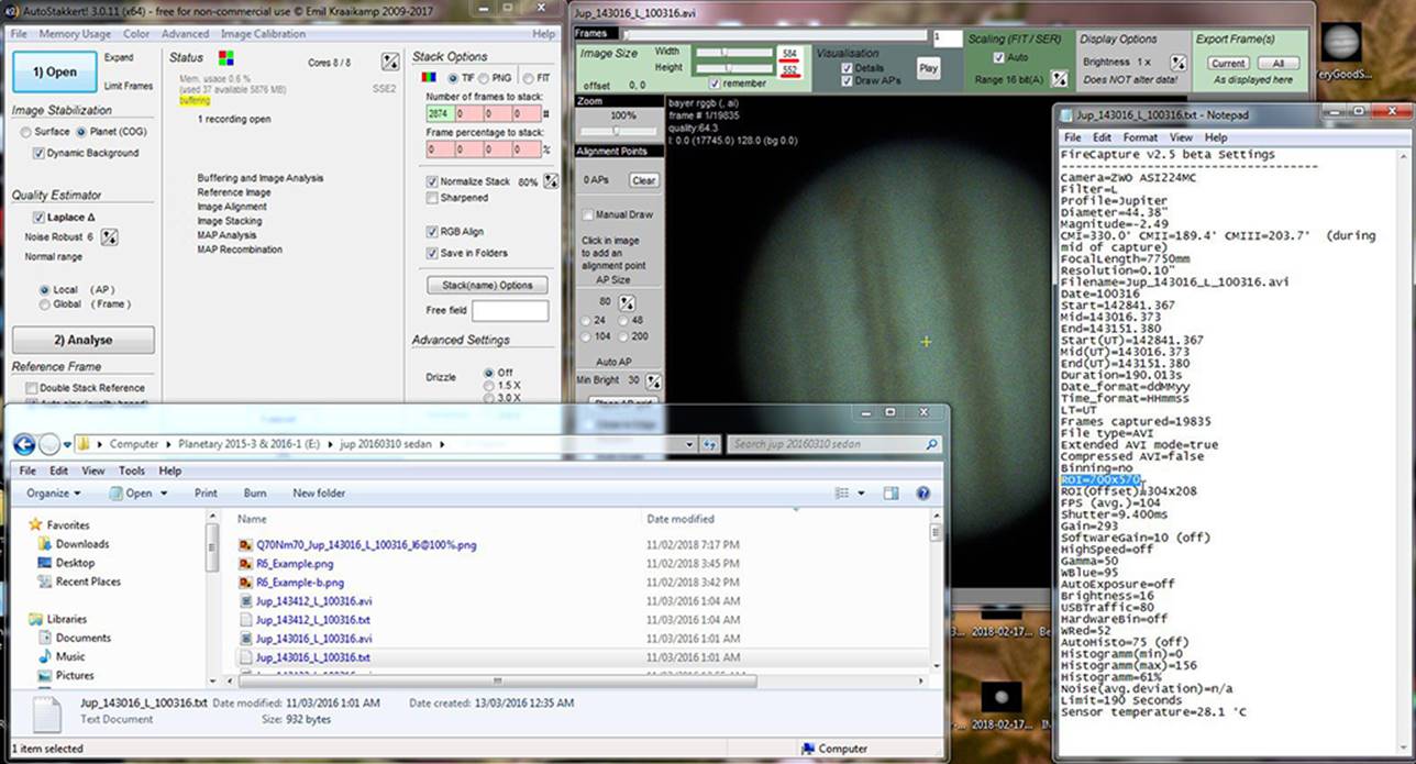
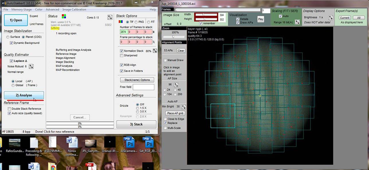
Once we have captured the avi (this is 8-bit, the planets never require more than 8-bit acquisition to be blunt!) we load the file into AutoStakkert. (AS!3 or AS!2) as per the image above. It is a simple "drag & drop" procedure & you can also see that I have opened the FireCapture .txt file showing that we used a 700x570 pixel ROI to capture Jupiter - this is important when setting the "Image Size Width & Height" underlined in red for the "Background" in AS!3. You need a bit of space around the planet to allow the MAPs boxes to overlap the planet's edges (more if moons were captured) but you are advised to not have any red screen displayed when setting this background size. In practise I have found that the occasional small amount of red background at the edges of some frames is of no consequence. You will also need to check that "Auto Detect" is enabled in the dropdown window under "Color" or even "possibly" "Force" the correct colour combination, usually "rggb." |
|
|
|
|
|
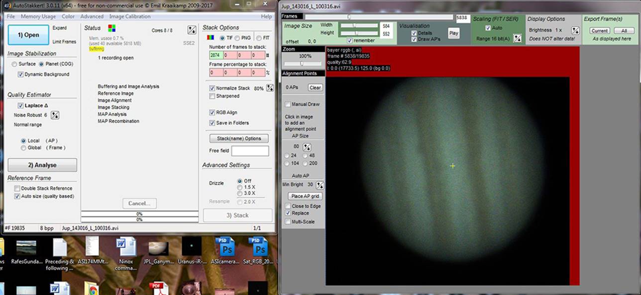
Here you can see I have "scrolled" through the frames using the pointer at the top of the RHS window (underlined in red area) & found a frame which not only shows a large amount of red background, but the planet itself has been cut! This is due to poor Polar Alignment & my habit of letting the planet drift around onscreen somewhat during capture - this has a reason behind it but in this case it was way too much drift! ;) AS!3 is meant to throw out these sorts of frames but in practise this isn't always the case. You can see from the details in that window that this was "frame # 5838/19835" |
|
|
|
|
|
To manually delete this "bad frame" you simply press the space bar on your keyboard with the frame selected, the above image showing what happens when you do this. (the text turns white etc indicating it has been removed from the stack) If you only have a few bad frames this is the simplest method of removing them. |
|
|
|
|
|
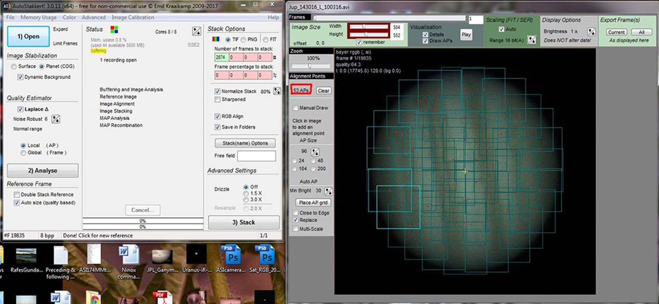
Time now to build your MAPs alignment box arrangement: I use a simple "wheel" arrangement that seems to work fine. The above image shows how I start this on Jupiter, first clicking on the yellow cross that appears at the centre of the screen/planetary disk. Choose sizes proportionate to the disk size - if you scale your boxes with a similar proportion (not size!) when comparing your own capture disk size you will not go wrong - in other words if your disk is only half the size of the one shown above make each of your MAPs boxes cover roughly only about 1/2 what these do here: in practise this means if these here are size "96" then a MAPs box roughly 1/2 this size is about "64"& not "48" which would only be about a 1/4 the area size & require many more boxes to cover the planet! I find the total of 53 boxes used here quite adequate usually. After the central MAP box is placed I then place 4 more around this & then another 8 around these as per the image above. |
|
|
|
|
|
I then place 16 more equi-spaced in a circle/wheel around the first lot as per the image above. |
|
|
|
|
|
Finally I place another 24 around those, trying to keep each box reasonably equi-spaced wrt each other's centre point but not too concerned, as I suspect (without any real evidence lol) that a bit of randomness is a good thing! ;) The only admonition is to keep each of their centres well back from the edges of the planet for this last set: the 53 MAPs boxes at size "96" is I believe is quite sufficient for this sized Jove - if your planet images are smaller you could have the same number of boxes but use smaller size MAPs than the above. |
|
|
|
|
|
On the left in the left-hand window you will need to check the
"Laplace" option for "Quality Estimator" & have
"Noise Robust" at "6" which is the default here. Also
make sure the "Color" tab dropdown is
selected to "AutoDetect" or "Force ----" & then hit
"Analyse." (if you haven't
set the "Color" tab correctly, the
planet's image will not appear as a colour image!) |
|
|
|
|
|
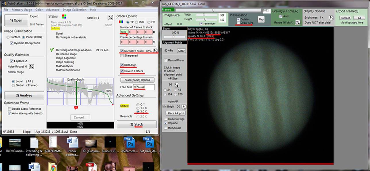
Here we see the results of AS!3's analysis in the graph, it has also ordered all the frames in the avi into a contrast-estimated quality order starting with what it has determined to be the best frame through to the worst based upon contrast-variation. (which is a good measure of the amount of light & dark detail on the planet's disk.) You can see that there was a dip in the quality of the images in the avi about 3/4 way along in the recording. |
|
|
|
|
|
If you use the scroll-bar (see 5th image from top) you can see the quality variation as you scroll to the right: you will also see the quality of any frame in the top left of the background in the right hand window expressed as a % compared to the best frame, which is rated at 100%. I have stopped at frame #8812 which is rated at 65% of the best frame's quality - a quite reasonable number of frames (8812) & quality cut-off at 65% or better compared to the best frame. You will notice I like to uncheck the "Draw AP's" checkbox so I can clearly see each frame to give me a better feel for the quality of the frames I am about to include in the stack I'm about to trigger - you'll also see a vertical green line that moves correspondently in the "Analysis" graph as I shift the scroll bar, this shows in graphic form the "#8812/19835 @ 65%" I have spoken about here. I then type this 8812 into the self-explanatory "Number of frames to stack" box as well as checking the "Normalize Stack" & setting a % value here: this adjusts the brightness of each frame in the stack about to be created to (in this case) 80% of the brightness of the brightest frame present. (unless seeing is almost perfect you will notice that during any recording you capture, the brightness of the onscreen feed will fluctuate noticeably throughout) Also check the "RGB Align" & the "Save in Folders" boxes & I like to put a note in the "Free Field" box for reference sake later: here I placed "Q65Nm80" which will appear at the beginning of the file-name of the stack about to be created - this signifies that I have chosen all frames 65% & above & set the "Normalize Stack" at 80%. Below this I have checked the "Drizzle - 3x" bullet box, this is a good option to try if your recordings are of sufficient quality...otherwise check the "Off" or possibly the "1.5x" which only halves the 3x output at the end of the stacking process anyway. ;) You can do this halving scale reduction in Registax6 & avail yourself of the various filters when reducing the size of the images in the stack by doing it there, so I'd suggest using either "Off" or "3x" in AS!3. Next Hit "Stack" |
|
|
|
|
|
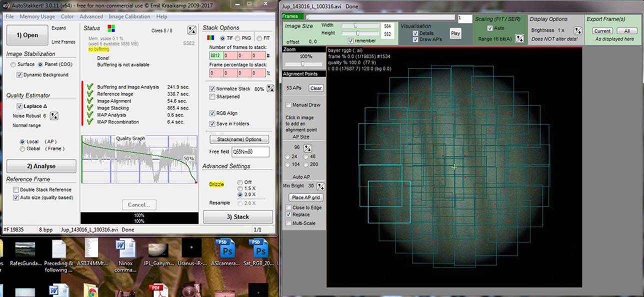
You can see that there are green ticks alongside each of the different processing stages, indicating processing has finished & the stack has been created. :) |
|
|
|
|
|
|
|
|
Above we see the file that AS!3 has created in the folder you loaded the avi from, as well as the RAW (unsharpened) stack that AS!3 created in the 2nd image just above. (slightly brightened for clarity) |